
This is a method for fuzzy search (extraction) with the FILTER function.
What is the FILTER function?
You can use the FILTER function to extract the result of a specific condition from within a range.
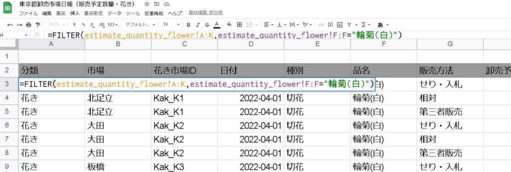
=FILTER(array, contains, [if empty])By using the FILTER function of Google Sheets, you can extract the result of the specified value from the table.
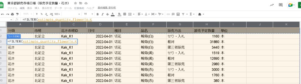
I was able to extract the ring chrysanthemum (white) in row F.
Is fuzzy search not possible with the FILTER function?
Even if you try to do a fuzzy search with this filter function, the result will not be returned as it is. Is it possible with asterisk? And even if I try, it will return an error (no matches).
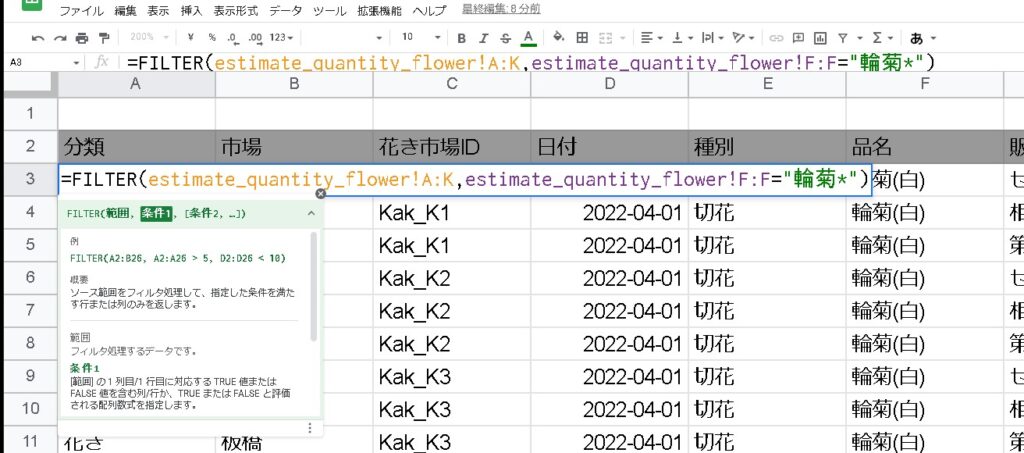
=FILTER(estimate_quantity_flower!A:K,estimate_quantity_flower!F:F="輪菊*")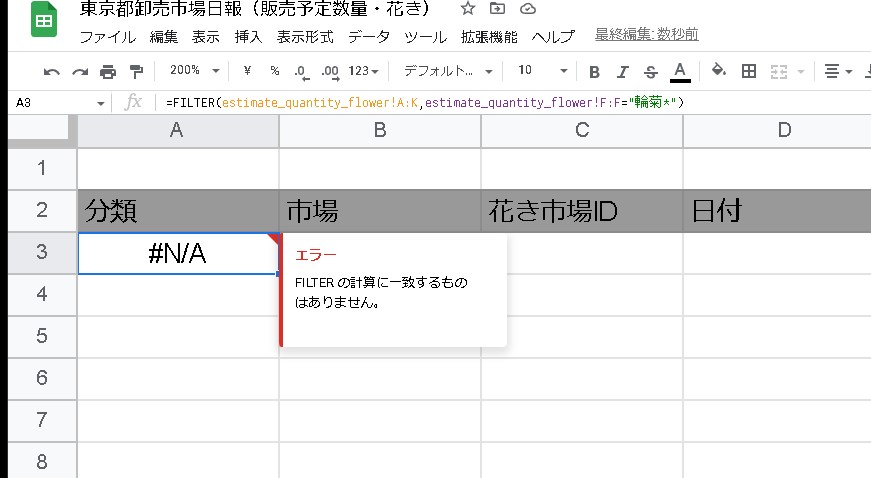
In this case, it is a method to realize a fuzzy search.
Combining FIND functions
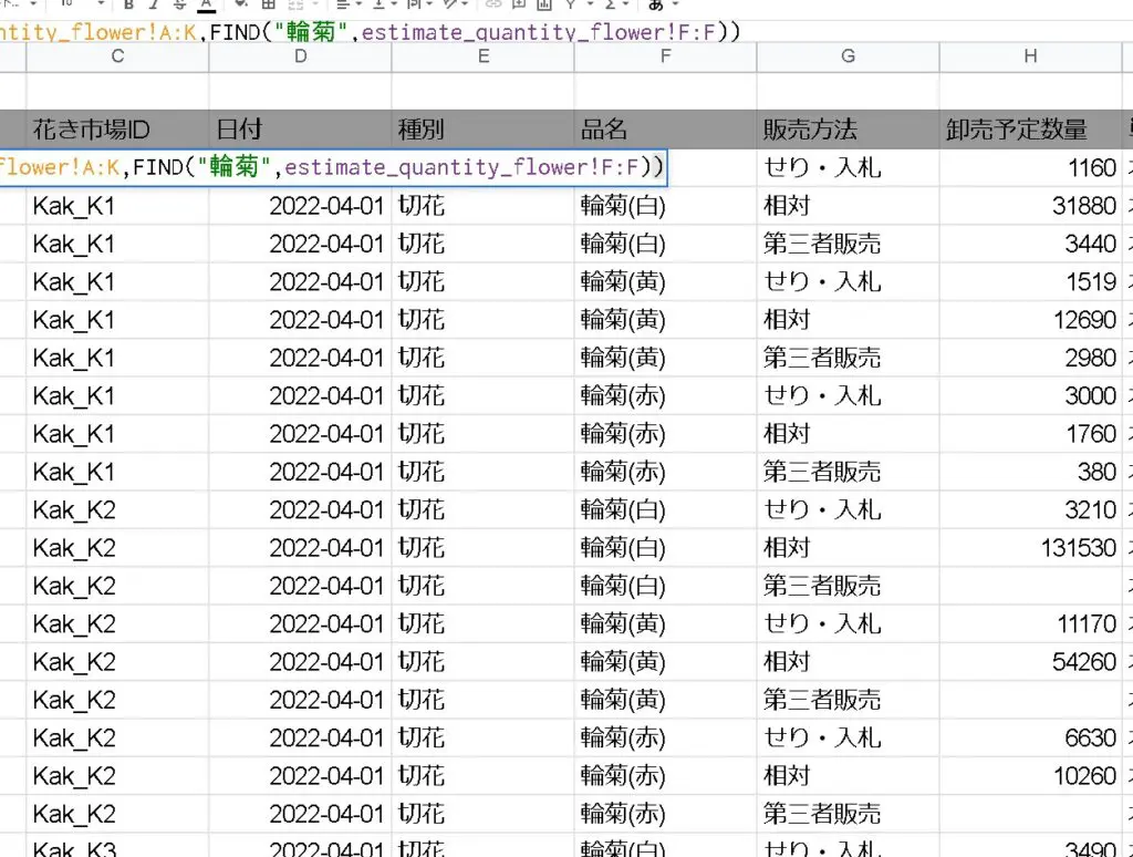
Now combine the FIND function.
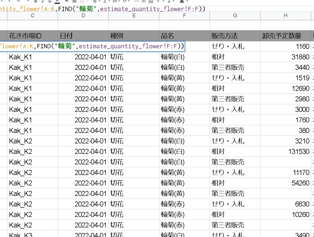
=FILTER(estimate_quantity_flower!A:K,FIND("輪菊",estimate_quantity_flower!F:F))The fuzzy search returned results!
summary
Combining the FIND function with the FILTER function changed it to “contains”.
Why is the return value of the FIND function like this…? is a mystery at the moment, but by combining the FILTER function and the FIND function, it is possible to extract fuzzy filters.
Please refer to it.